Ground state calculation

quantum_groundstate

extern double quantum_groundstate(quantum_reg *reg, double epsilon, quantum_reg H(MAX_UNSIGNED, double), int solver, double stepsize);

This function returns the ground state energy of the Hamiltonian implemented in the function H. The quantum register reg should have been initialized with quantum_new_qureg_size and filled with random amplitudes for best results. Upon return, reg will contain the ground state of the Hamiltonian. The desired absolute precision of the energy is controlled with epsilon. The variable solver allows to choose from different algorithms and can take any of the following values:

Value	Description
QUANTUM_SOLVER_LANCZOS	A straight-forward implementation of the Lanczos algorithm. As this implementation does not perform reorthogonalization, results may become unreliable for very large system sizes.
QUANTUM_SOLVER_LANCZOS_MODIFIED	A modified (and slower) version of the Lanczos algorithm [Dagotto, 1985] that is numerically stable.
QUANTUM_SOLVER_IMAGINARY	Imaginary time evolution using quantum_rk4.

Generally speaking, QUANTUM_SOLVER_LANCZOS is the fastest algorithm, but QUANTUM_SOLVER_LANCZOS_MODIFIED and QUANTUM_SOLVER_IMAGINARY are more reliable. Finally, the variable stepsize only needs to be supplied for QUANTUM_SOLVER_IMAGINARY and should correspond to the inverse of the typical energy scale of the Hamiltonian. Note that using the ground state solver will almost certainly require the use of double-precision arithmetic, which can be enabled by the --with-complex-type="double _Complex" configure switch.

Example: Transverse Ising chain

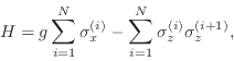
The transverse Ising chain in a one-dimensional spin $1/2$ model is described by the Hamiltonian

$$H = g\sum\limits_{i=1}^N \sigma_x^{(i)} - \sum\limits_{i=1}^N \sigma_z^{(i)}\sigma_z^{(i+1)},$$

where $\sigma_\alpha^{(i)}$ refers to the Pauli spin matrix acting on the $i$th spin,$N$ is the total number of spins and $g$ is the magnitude of the external field in the transverse direction given in units of the ferromagnetic Ising interaction between the spins. Here, we are interested in periodic boundary conditions, i.e., $\sigma_\alpha^{(N+1)} = \sigma_\alpha^{(1)}$. This Hamiltonian exhibits a quantum phase transition at the critical field $g_c = 1$ from a ferromagnetic ($g<1$) to a paramagnetic ($g>1$) phase [Sachdev, 1999]. The ising demo program supplied with libquantum calculates the ground state $\vert\psi_0\rangle$ and its spontaneous magnetization

$$m = \langle \psi_0 \vert \left\vert\sum\limits_{i=1}^N \sigma_z^{(i)} \right\vert \vert\psi_0\rangle$$

for various values of $g$ and different system sizes. From the theory of finite-size scaling [Cardy, 1996], it is known that close to the critical point, $m$ has to behave like

$$m = N^{-\beta/\nu}\tilde{m}\left([g-g_c]N^{1/\nu}\right),$$

where $\tilde{m}$ is a rescaled magnetization function and $\beta$ and $\nu$ are the critical exponents of the phase transition. Fig. 1 shows that plotting the magnetization data in a rescaled fashion causes all data points to collapse onto a single line. We can also use this data collapse to numerically extract values for $g_c$ and the critical exponents. Here, we find $g_c = 0.997\pm 0.005$, $\beta=0.122\pm 0.006$, and $\nu = 1.03\pm 0.02$, which is in very good agreement with the exact values of $g_c = 1$, $\beta = 1/8$, and $\nu=1$.

Figure 1: Data collapse in the finite-size scaling for the transverse Ising chain ($g_c=0.997$, $\beta = 0.122$, $\nu = 1.03$).